Option Pricing – ESE 303

Black-Scholes model of option pricing

**Figure 1**. Price of Cisco (CSCO) between November 25, 2008 and November 24, 2009. Stock prices can be modeled as a geometric Brownian motion.

Consider a public company with stock price $X(t)$ at time $t$ . A European style option on the stock of this company is a contract to have the option to buy the stock at a predetermined price on a predetermined future time. The option is described by the strike price $K$ , the strike time $t$ and its price $c$ . Paying $c$ to buy an option gives us the opportunity to buy the stock for the strike price $K$ at the strike time $t$ . At time $t$ , the worth of the option depends on the value of the stock $X(t)$ . If the stock has fallen below the strike price $K$ , i.e., if $X(t)\leq K$ the option becomes worthless because it is more convenient to pay the actual price $X(t)$ for the stock and forgo the option. If, on the contrary, the price has risen beyond $K$ , i.e., if $X(t)>K$ we can realize a gain $X(t)-K$ by exercising the option to buy the stock at price $K$ . This gain can be cashed immediately by reselling the stock at the current price $X(t)$ . We can thus write the worth $w$ of the option as

$w = \big[X(t) - K\big]^{+},$

where $(x)^{+} = \max(0,x)$ denotes projection on the positive numbers.

The gain to be realized by the trading strategy “buy option at time $t=0$ , exercise the option at time $t$ if $X(t)>K$ , sell stock at price $X(t)$ ” depends on the difference between $w$ and $c$ . It is not exactly the difference because it is not equivalent to own $c$ at time $0$ and $c$ at time $t$ . In particular, while the proposed investment strategy incurs some risk of loosing the initial investment $c$ , it is possible to invest $c$ in a risk-free money market account. If the interest in the money market account is $\alpha$ continuously compounded, the worth of the money market investment at time $t$ is $ce^{\alpha t}$ . Consequently, when comparing investment and payoff it is fairer to compare $w$ with $ce^{\alpha t}$ because growing $c$ to $ce^{\alpha t}$ is literally effortless. Equivalently, we can compare $c$ to $we^{-\alpha t}$ because capital $we^{-\alpha t}$ at time $0$ can be grown to $w$ at time $t$ through a risk-free money market investment. The latter comparison is the one commonly used and, in general, we say that a capital $w$ at time $t$ has a present value or a time-zero value of $we^{-\alpha t}$ . We may also refer to $we^{-\alpha t}$ as the discounted worth. Using the option’s worth expression, we can compute the discounted gain of an option investment as

$w = e^{-\alpha t}\big[X(t)-K\big]^{+} - c .$

The relevant question here is what is a fair price $c$ for an option with strike price $K$ to be exercised at time $t$ . The answer to this question is given by the Black-Scholes formula for option pricing that uses expectations on the future behavior of the stock to determine the option’s price $c$ . To understand Black-Scholes formula, we need to introduce the Geometric Brownian motion model of stock prices, discuss the concept of arbitrages, and define risk neutral measures. The geometric Brownian motion model of stock prices is presented next. For arbitrages and the risk neutral measure you’ll have to wait for the class.

Geometric Brownian motion model of stock prices

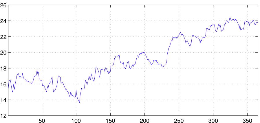
It suffices to examine a graph with the evolution of a stock price, e.g., Fig. 1, to realize that stock prices are, to some extent, random. To construct a stochastic model of stock prices, notice that variations in a stock price are likely to be proportional to the price of the stock $X(t)$ . That is, if the price of the stock is $X(t)=10$ , a variation of plus or minus $1$ is akin to a variation of plus or minus $10$ , when the price is $X(t)=100$ . A particular class of stochastic processes with such property is geometric Brownian motion (GBM). This model presupposes that relative variations on the price $X(t)$ can be described as a Brownian motion with drift. Specifically, it assumes that changes in prices are according to the expression

$X(t+s) = X(t) e^{Y_{t}(s)}$

where $Y_{t}(s)$ is normally distributed with mean $\mu s$ and variance $\sigma^{2}s$ independently of $s$ . Definition of a GBM also requires relative price changes $Y_{t_{1}}(s_{1})$ and $Y_{t_{2}}(s_{2})$ in disjoint time intervals to be independent. In the context of stock pricing, the mean $\mu$ represents the stock’s drift and the variance $\sigma^{2}$ its volatility.

An equivalent characterization of a GBM is to state that a process $X(t)$ is a GBM if its logarithm $\log X(t+s)$ is a regular Brownian motion (BM) with drift. Indeed, taking logarithms in both sides of the previous equation yields

$\log X(t+s) = \log X(t) + Y_{t}(s)$

The two conditions imposed on $Y_{t}(s)$ , namely that $Y_{t}(s)$ is normal with mean $\mu s$ and variance $\sigma^{2}s$ and that $Y_{t_{1}}(s_{1})$ and $Y_{t_{2}}(s_{2})$ are independent for disjoint time intervals, along with the relationship just derived imply by definition that $\log X(t)$ is a BM.

An important observation to make here is to consider a discretization in time steps of fixed duration $h$ , say $h=1 \text{ day}$ , and to define the discrete time stochastic process $Y_{n}$ as

$Y_{n} := \log X(nh) - \log X\big((n-1)h\big) = Y_{(n-1)h}(h)$

It follows from the GBM model, that variables $Y_{n}$ are independent identically distributed normals with mean $\mu h$ and variance $\sigma^{2}h$ . This is an important observation because it allows us to infer the parameters $\mu$ and $\sigma^{2}$ from empirical data. Indeed, let it be available a historic sequence of stock prices $x(nh)$ for $n=0,\ldots,N$ , taken from a realization $x(t)$ of the GBM stochastic process $X(t)$ . From $x(nh)$ we compute $y_{n}=x(nh)- x \big(n(h-1)\big)$ to obtain a realization of the stochastic process $Y_{n}$ . The drift parameter $\mu$ can then be estimated by the sample mean

$\hat{\mu} = \frac{1}{Nh} \sum_{n=1}^{N} y_{n} ,$

and the volatility parameter $\sigma$ can be estimated by the sample variance

$\hat{\sigma}^{2} = \frac{1}{(N-1)h} \sum_{n=1}^{N} \left(y_{n}-\hat{\mu}\right)^{2} .$

While we have given a justification for why GBM is a plausible model for stock prices, the actual motivation for their use, is that GBM models have been observed to provide reasonable fits of empirical stock price sequences. This fit is easy to observe using drift and volatility estimates $\hat{\mu}$ and $\hat{\sigma}^{2}$ computed from empirical data. If a GBM with drift $\hat{\mu}$ and volatility $\hat{\sigma^{2}}$ is a good model for the evolution of a stock price, then the variables $Y_{n}$ have a probability density function (pdf) $N\left(\hat{\mu}h,\hat{\sigma}^{2}h; y\right)$ . We can then estimate the pdf of $Y_{n}$ using a histogram of the $y_{n}$ and compare it with the pdf $N\left(\hat{\mu}h,\hat{\sigma}^{2}h; y\right)$ .

As a particular example, consider the stock price of Cisco during the year 2009 depicted in Fig. 1. More recent data for this stock and others is publicly available, see, e.g. Google finance. The comparison between the normal pdf $N\left(\hat{\mu}h,\hat{\sigma}^{2}h; y\right)$ and the histogram of $y_{n}$ is shown in Fig. 2. A comparison between the cumulative distribution function (cdf) and the empirical cdf is also shown. From either picture a reasonable fit between model and observations is seen.

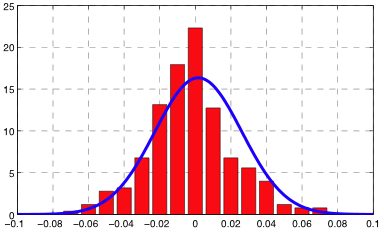
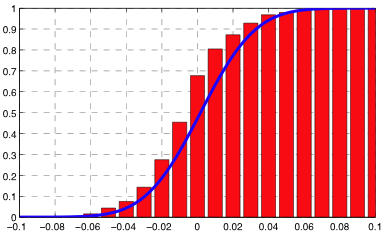
Figure 2. Fit of Cisco’s stock price (CSCO) to geometric Brownian motion (GBM) model. If GBM is a good model of stock price variations, the relative changes in stock prices from closing date to closing date are independent identically distributed normal random variables. Empirical probability distribution function (left) and cumulative distribution function (right) of CSCO relative changes in closing price are compared with a normal random variable. From either picture a reasonable fit between model and observations is seen.